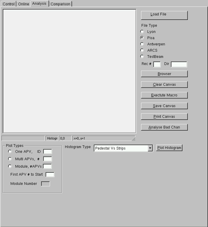
• Open File : A root file can be loaded using "Load File" button. This button would activate a "Dialog" to select file name.
• File Type : The type of the root file (Outputs from HybridDialog/Pisa Client/Lt Client/ARCS Client/Beam Test[GeneralTT6.cpp]) should be specified in the "Radio Button" after loading the file. In case of Pisa Client if more than 4 APVs are present on can specify "Starting APV Number" in the corresponding "Text Field" labeled as "First APV # to Start" . In case of Beam Test output one MUST specify the "Module Number" .
• Rec# and Dir: The directory structure in the root file should be specified here. In case of Lt Client/ARCS Client the directory structure contains a record (with a given number) and then under that, directories like PeakInvOn, PeakInvOff, DecInvOn and DecInvOff depending on the APV mode of data taking are saved. One has to specify it here to select corresponding histograms. There are two "Text Fields" and once has to specify the number of the record and Directory Name.
• Root Browser : Using "Browser" button one can open a "TBrowser" from ROOT. Any histogram from the TBrowser can be plotted into the "Embedded Canvas".
• Clear Canvas : The "Embedded Canvas" can be cleared using "Clear Canvas" button.
• Execute Macro : Any macro file suitable to the root file opened, can be executed by clicking the "Execute Macro" button. To plot in the "Embedded Canvas" one needs to specify the name of this canvas "Histogram Canvas" otherwise one can define separate "TCanvas" in the macro. There are a number of macros in the 'macro' directory of the software but they can not be invoked using "Execute Macro" as they are used internally from the software to plot different types of histograms.
• Save Canvas : Once one/more histograms are plotted in the "Embedded Canvas", the picture can be saved in postscript format using "Save Canvas" button.
• Print Canvas : The plots in the "Embedded Canvas" can be directly printed in a printer using "Print Canvas" button. This would activate a dialog where the printing command should be specified. But before using this button one MUST make sure the printer is properly configured and is usable from the PC.
• Analyse Bad Chan : The channels are identified from bad "Noise", "Pulse Height", "Peaking Time" behaviors. The resulting histogram is plotted in the "Embedded Canvas" . a detailed explanation is given below.

There are three different ways to plot histograms. A specific type can be selected in the "Plot Types" frame. The available options are,

• One APV at a Time : one needs select "One APV" check button and specify APV number in the adjacent text-field. The numbering should be starting from ONE and not from ZERO.
• More Than One APV at a Time : the "Multi APV" check button should be selected and number of APVs should be specified in the adjacent text field.
• As a Module : The "Module " check button should be selected and # of APVs in the module is to be specified in the text field.
• Starting APV # : If more than 4 APV's are analysed one should specify the APV # to start with in the "Text Field". This is required for the plotting using "More Than One APV at a Time"/"As a Module" options.

The histogram to be plotted can be selected in the "pull down menu", "Histogram Type". The list of the quantities are

1. Pedestal Vs Strips

2. Pedestal Distribution

3. Raw Noise Vs Strips

4. Raw Noise Distribution

5. Noise Vs Strips

6. Noise Distribution

7. Common Mode Distribution

8. Calibration Charge vs Strip

   [this is the calibration charge at a fixed latency. This histogram is not available from ARC client]

9. Calibration Charge Distribution

10. Calibration Profile with Time

    [can ONLY be plotted for "One APV at a Time" or "More Than One APV at a Time". Can not be plotted in Module Option]

11. Channel Flag vs Strip

12. Channel Flag

13. Maximum Charge Vs Strips

14. Maximum Charge Distribution

15. Rise Time Vs Strips

16. Rise Time Distribution

17. Data-Pedestal-CM vs Strips

18. Data-Pedestal-CM Distribution

19. Laser Pulse vs Strip

20. Number of Cluster

21. Number of Cluster

22. Cluster Charge

23. Cluster Position

24. Cluster Width

25. Cluster Noise

26. Eta Function

27. Cluster Shape

28. Temperature vs Time

29. Hybrid Current vs Time

30. Leakage Current vs Time

Aanalysing Bad Channel :
A channel is defined bad from its Noise, Pulse Height, and Peaking Time behaviors as defined in the Torino Workshop in July 2003. See Talk by Cristiano The cuts used here and the corresponding Badness Flags are the following :

1. Noise Cut (absolute):
   
   • Peak Mode : 0.95 < Noise < 1.45
   • Deconvolution Mode : 1.3 < Noise < 2.0
   If a strip is outside this specification the flag value is assigned as +2 (above upper cut) and -2 (below lower cut) and is plotted in red
   
2. Pulse Height Cut (in percentage wrt the mean):
   
   • Peak Mode : +- 15%
   • Deconvolution Mode : +- 20%
   If a strip is outside this specification the flag value is assigned as +4 (above upper cut) and -4 (below lower cut) and is plotted in Green
   
3. Peaking Time Cut (absolute):
   
   • Peak Mode : +5 ....-5
   • Deconvolution Mode : -3 .... +5
   If a strip is outside this specification the flag value is assigned as +6 (above upper cut) and -6 (below lower cut) and is plotted in Blue